
How to Reduce LLM Inference Cost: 7 Levers That Move the Number
LLM inference cost is the total compute, memory, networking, and operations spend required to generate tokens in production, and it is usually driven by utilization, batching, model size, and infrastructure choice rather than raw GPU price. Teams that lower per-request cost rarely do it by negotiating hardware discounts; they change how requests are batched, how memory is allocated, and which model serves which query.
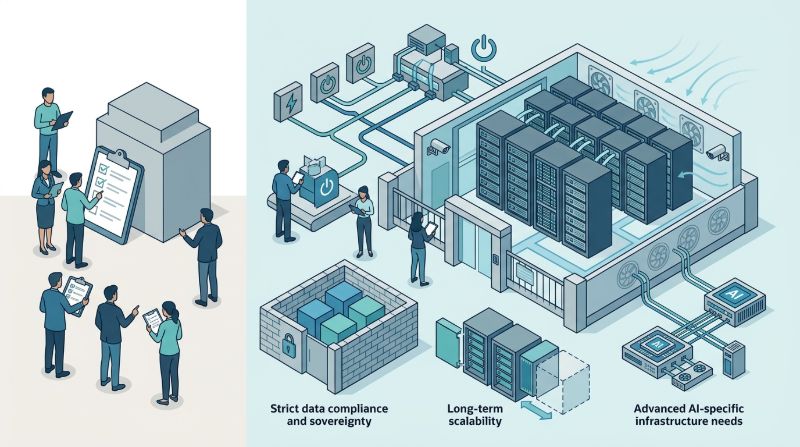
For enterprise teams, inference cost is the line item that scales fastest as usage grows. A model that costs cents per request in testing can become the largest infrastructure bill in production once traffic, concurrency, and latency targets compound. Reducing it is a systems problem, not a procurement problem.
This guide walks through seven levers that reliably move inference cost, what each lever trades off, and how to sequence them so improvements compound instead of canceling each other out.
What Actually Drives LLM Inference Cost
Before tuning anything, isolate where cost is generated. Inference cost breaks down into four components, and the dominant one varies by workload. A team optimizing the wrong component sees no improvement and concludes inference is just expensive.
The four cost drivers are compute (GPU seconds spent generating tokens), memory (GPU memory held by weights, KV cache, and active requests), networking (node-to-node traffic in multi-GPU or multi-node serving), and operations (idle capacity, monitoring overhead, and staff time). For most workloads, memory and utilization, not peak compute, dominate. A GPU at 100% peak utilization for two seconds is cheaper than the same GPU at 20% utilization for ten seconds, even though both produce the same output.
Measure Cost per Token Before Optimizing
Establish a baseline metric before changing anything. Cost per 1,000 tokens (input plus output) is the most useful unit because it normalizes across request sizes and model variants. Track it alongside throughput (tokens per second) and tail latency (p95 or p99), because cost reduction that destroys latency is not a reduction, it is a service degradation.
A common mistake is optimizing for average latency while p95 latency silently grows. Users notice the slow tail, not the fast average. Always pair any cost change with a latency and quality regression check.
Lever 1: Increase Batch Utilization
Batching is the single highest-impact lever for most serving workloads. A GPU generating tokens for one request at a time wastes most of its parallel capacity. Batching multiple requests together keeps the GPU saturated, which means the same GPU-seconds produce more tokens.
Continuous batching (also called iteration-level batching) is the current standard because it admits and evicts requests mid-generation rather than waiting for a batch to complete. For teams running conversational or streaming workloads with variable request lengths, continuous batching typically improves throughput substantially over static batching. The tradeoff is implementation complexity and slightly higher tail latency when the batch is full.
Right-size the maximum batch size against GPU memory. Too small leaves capacity unused; too large triggers memory pressure, eviction, and retry storms that cost more than they save. Tune empirically under real traffic, not synthetic benchmarks.
Lever 2: Quantize the Model
Quantization reduces the precision of model weights and activations, which shrinks memory footprint and increases the number of tokens a single GPU can generate per second. Moving from FP16 to INT8 or INT4 can cut memory requirements and improve throughput meaningfully, lowering cost per token.
The tradeoff is quality and calibration effort. Lower precision can degrade output quality on edge cases, and poorly calibrated quantization causes larger quality drops than benchmarks suggest. Test quantized models against a held-out evaluation set that reflects real user queries, not just standard benchmarks. For many enterprise workloads, well-calibrated INT8 is indistinguishable from FP16 for users, while INT4 is viable for retrieval, classification, or first-pass ranking where perfect fidelity is not required.
Lever 3: Right-Size KV Cache and Context
The KV cache holds intermediate attention state for each active request and grows with context length. For long-context workloads, KV cache memory can exceed the memory used by model weights. Left unmanaged, it caps concurrency, forces more GPUs, and inflates cost per token.
Three controls help. First, cap maximum context length to what users actually need; generous defaults often exceed real usage and pre-allocate memory that goes unused. Second, evict or compress KV cache for idle or completed requests rather than holding it. Third, use paged or chunked attention mechanisms that allocate KV cache dynamically instead of reserving worst-case memory per request. These changes directly increase how many concurrent requests a fixed GPU pool can serve, which is equivalent to lowering cost per request.
Lever 4: Route to the Cheapest Sufficient Model
Not every request needs the largest model. Routing simple queries to a smaller, faster, cheaper model and reserving the large model for complex or high-value requests can cut aggregate cost substantially. This is model routing, sometimes called cascade or hierarchical serving.
Implementation ranges from simple rules (route by input length, detected intent, or user tier) to learned routers that predict which model will produce an acceptable response. The tradeoff is complexity in the routing layer and the risk of quality variance when the router misclassifies a query. Start with coarse rules, measure quality with human or automated evaluation, and refine. For teams with mixed workloads, this lever often delivers the largest single cost reduction after batching.
Lever 5: Use Speculative Decoding Where It Fits
Speculative decoding uses a small draft model to propose tokens that the large model verifies in parallel. When the draft model is accurate, the large model accepts multiple tokens per forward pass, increasing throughput without changing output quality. For workloads with predictable, repetitive, or structured outputs, the throughput gain is significant.
The lever does not fit everywhere. It adds a draft model to operate, it can hurt latency on single-request low-batch paths, and it underperforms when outputs are highly creative or unpredictable. Profile before adopting, and treat it as a complement to batching, not a replacement.
Lever 6: Match Infrastructure to the Workload Pattern
Infrastructure choice sets the floor on cost. Spot or preemptible GPU capacity is cheap but unsuitable for latency-sensitive or stateful serving because instances disappear without warning. On-demand public cloud GPU is flexible but priced at a premium that compounds at scale. Dedicated GPU clusters, whether owned or leased, have a higher fixed cost but a much lower marginal cost per token once utilization is high.
The decision hinges on utilization and predictability. Teams with steady, high traffic and latency commitments usually find dedicated infrastructure cheaper at scale, because they pay for capacity rather than per-request volatility. Teams with bursty, unpredictable, or experimental traffic often do better on flexible capacity. For teams evaluating this tradeoff, providers with US-based dedicated GPU environments and managed operations, such as OneSource Cloud's Private AI Infrastructure, offer a middle ground: predictable capacity without the operational burden of self-managed clusters.
Lever 7: Cut Idle and Over-Provisioned Capacity
Idle GPU time is pure cost. Many serving deployments over-provision to handle peak traffic or latency spikes, then run at low average utilization the rest of the time. The gap between peak and average utilization is where most wasted spend hides.
Controls include autoscaling that tracks real queue depth rather than fixed thresholds, scheduled scaling for known traffic patterns, and load shedding or graceful degradation under spikes instead of holding spare capacity permanently. Pair these with the monitoring covered in the next section. Reducing idle capacity is unglamorous, but it is often the fastest win because it requires no model changes, only operational discipline.
Cost Levers Comparison
| Lever | Typical impact | Main tradeoff | Where to start |
|---|---|---|---|
| Batch utilization | High | Implementation complexity, tail latency | Enable continuous batching, tune batch size |
| Quantization | Medium to high | Quality on edge cases, calibration effort | INT8 on a held-out eval set |
| KV cache and context | Medium | Eviction logic, max-context policy | Cap context, enable paged attention |
| Model routing | High for mixed workloads | Router complexity, quality variance | Route by intent or input length |
| Speculative decoding | Medium, workload-dependent | Draft model overhead, single-request latency | Profile on structured outputs |
| Infrastructure match | High at scale | Commitment vs flexibility | Compare dedicated vs on-demand by utilization |
| Idle capacity reduction | Fast win | Operational discipline, autoscaling tuning | Right-size to average, autoscale to peak |
Sequencing the Levers
Apply the levers in an order that compounds. Start with measurement (cost per token, throughput, p95 latency), then batching, because it amplifies every later lever. Next, address memory (quantization and KV cache), which increases how much each GPU can hold and serve. Then layer routing and speculative decoding, which change how requests map to models. Finally, revisit infrastructure and idle capacity, which set the cost floor. Skipping measurement and jumping straight to a single lever is the most common reason cost reduction efforts stall.
Monitoring Signals That Catch Cost Regression
Cost optimization is not a one-time project; without monitoring, savings erode as traffic, models, and prompts drift. Track these signals continuously:
- Cost per 1,000 tokens, segmented by model and route, to catch per-request drift early.
- GPU utilization average versus peak, to spot idle capacity and over-provisioning.
- Queue depth and time in queue, to detect saturation before it forces more GPUs.
- Eviction and retry rates, which signal memory pressure or batch misconfiguration.
- Quality metrics on a fixed eval set, to catch silent degradation from quantization or routing.
For teams that want a consolidated view, an AI operations platform that surfaces token-level latency, utilization, and cost together — such as the OnePlus Platform for orchestrating GPU capacity and model serving — helps correlate cost changes with the lever that caused them.
FAQ
How much can I reduce LLM inference cost?
It depends on the starting point, but teams that have never tuned batching or quantization often cut cost per token substantially. The largest single gains usually come from continuous batching and model routing. After those, returns flatten and require more engineering effort. Always measure cost per token before and after each change so gains are real, not assumed.
Does quantization hurt model quality?
Well-calibrated INT8 quantization is often indistinguishable from FP16 for typical user queries, while INT4 can degrade quality on edge cases or reasoning-heavy tasks. The key is testing on an evaluation set that mirrors real usage, not just public benchmarks. Treat quantization as a quality-cost dial tuned per workload, not a universal setting.
Is dedicated GPU infrastructure cheaper than public cloud for inference?
It depends on utilization and traffic predictability. Dedicated clusters have a higher fixed cost but a lower marginal cost per token once utilization is high, which makes them cheaper at steady, high-volume scale. Public cloud on-demand GPU wins for bursty or experimental traffic where paying per request is cheaper than holding capacity. The break-even point is workload-specific and worth modeling rather than assuming.
What is the fastest way to lower inference cost?
The fastest wins usually require no model changes: enable continuous batching, cap maximum context to what users actually need, and right-size capacity to average utilization while autoscaling for peaks. These three often reduce waste immediately. Deeper savings from quantization, routing, and speculative decoding follow once measurement is in place.
How does model routing reduce cost?
Routing sends each request to the cheapest model that can produce an acceptable response, reserving large models for complex queries. For workloads mixing simple and complex requests, aggregate cost drops because most traffic no longer hits the most expensive model. The tradeoff is router complexity and quality variance, which is why routing should start with coarse rules and an evaluation loop.
Summary
Reducing LLM inference cost is a systems problem solved by seven levers: batching, quantization, KV cache and context management, model routing, speculative decoding, infrastructure matching, and idle-capacity reduction. The order matters. Measure cost per token first, amplify every lever with batching, then attack memory, routing, and infrastructure in sequence. Teams that pair these levers with continuous monitoring — cost per token, utilization, queue depth, and quality — keep savings instead of watching them erode as usage grows.
For enterprise teams that want predictable per-token cost at scale, dedicated GPU infrastructure with managed operations removes the volatility that makes public cloud inference expensive at high utilization. Explore OneSource Cloud's private AI infrastructure to see how dedicated capacity and 24/7 operations support cost-stable LLM serving.
Related Articles
Recommended Reading
-
Google Cloud GPU Pricing: What Enterprise AI Teams Should Evaluate Before Provisioning
-
Paperspace Pricing 2026: GPU Cost Breakdown
-
CoreWeave Enterprise GPU Cloud: Evaluation for AI Teams
-
AI Infrastructure Costs: Controlling Enterprise GPU Spending
-
CoreWeave vs Lambda Labs: GPU Cloud Provider Comparison
latest articles
-
Open-Source LLM Deployment: Requirements and Real Cost Breakdown
-
AI Search Assistants Under Data Residency: Architectures and Evidence
-
LLM Inference GPUs Compared: A100, H100, H200, or B200 for Production
-
LLM Deployment Best Practices: An Enterprise Stage-by-Stage Checklist
-
HIPAA Patient Scheduling AI: Controls, Consent, and Evidence
-
Cloud-Agnostic LLM Deployment: Architecture Principles Against Lock-In
-
HIPAA-Compliant AI Tools for Healthcare: Categories and Evaluation
-
Batch vs Real-Time LLM Inference: Cost, Latency, and Fit
-
Model Deployment Strategies Compared: Canary, Blue-Green, Shadow, Rolling
-
GPU Rental vs Owning: Cost, Commitment, and When to Buy